Methods & Data Sources
This analysis was produced in a single week (June 2026) to support public understanding during the current European heatwave. If you spot errors or have suggestions, please flag them; they are genuinely welcomed. Contact: thami.croeser@gmail.com
Data pipeline
All analysis was conducted using open-source tools (Python, GDAL, GeoPandas) on publicly available datasets. The pipeline:
Tree canopy. Two sources, depending on availability. For eight cities (Berlin, Birmingham, Hamburg, Leeds, Liverpool, London, Munich, Newcastle): Google’s Environmental Insights Explorer (EIE) tree canopy layer at 0.2m resolution, accessed via Google Earth Engine (imagery predominantly 2022–2024, range 2020–2024). The EIE product uses machine learning to classify high-resolution aerial imagery into terrain types; pixels classified as “tree” form the canopy mask. For all other cities: Meta/WRI Global Canopy Height dataset (1m resolution, 2020 imagery), accessed via Google Earth Engine, with all detected vegetation included (no height filter applied). Nodata value set to 255 to prevent false-positive canopy counts at tile edges, a common issue with the Meta/WRI product where nodata pixels default to 0 and get counted as “no tree” rather than “no data”. Mosaics were computed per city from overlapping GEE export tiles, taking the maximum value at each pixel to handle tile overlaps. See Canopy resolution and height filtering below for detail on this methodological choice.
Building footprints. IGN BD TOPO v3 for French cities (accessed via WFS), Overture Maps Foundation for all other cities. Building height, type, and dwelling count from the same source where available. Overture Maps buildings were filtered to exclude non-building features (fences, walls, ruins) using the
classfield.Canopy per building. For each building, a 60m buffer was computed from the building outline polygon (not centroid) and the percentage of vegetation pixels within that buffer was extracted via windowed raster counting. No height filter is applied; all detected vegetation is counted as canopy (see All-vegetation canopy measure below). The 60m radius reflects the distance at which cooling from tree canopy has been shown to remain significant (Ziter et al. 2019). The
canopy_pct_60mmetric is the ratio of canopy pixels to total valid pixels within the buffer.Surface temperature. Landsat 8/9 Collection 2, Level 2 (ST_B10 thermal band), converted from scaled DN to degrees Celsius using the collection’s scale factor and offset. Scenes were manually selected during documented heatwave events for each city (see scene table below). Cloud-free scenes were prioritised; partial cloud cover was masked using the QA_PIXEL band. The temperature was then zonal-averaged per building footprint and per hex cell.
Income / deprivation. Country-specific indices at the finest available spatial resolution. Joined to buildings via spatial overlay. Variables were normalised to quartiles within each city to enable cross-country comparison despite different index methodologies.
Cool spots. Identified as hex cells (300m resolution) meeting three simultaneous criteria: mean canopy ≥20% within 60m, surface temperature below the city’s 25th percentile, and residential density ≥8 dwellings/ha. These represent dense urban areas that maintain adequate canopy and are measurably cooler.
Notable processing decisions
60m buffer, not building footprint. Canopy was measured within a 60m radius of each building, not within the building parcel. This captures street trees, small parks, and neighbouring gardens that contribute to localised cooling. The buffer distance is based on empirical evidence from thermal transect studies showing measurable cooling within ~50-80m of canopy clusters.
All-vegetation canopy measure. The analysis counts all detectable vegetation as canopy, without applying a minimum height threshold. This is a deliberate choice: cities that fall below the 30% canopy threshold even with this generous measure are almost certainly performing worse when only shade-providing mature trees are counted. Where the 0.2m product is available, it replaces the 1m product entirely. See Canopy resolution and height filtering below.
Nodata handling. The Meta/WRI canopy height product uses 0 for both “no tree” and nodata in some tiles. To prevent edge artifacts, all tiles were pre-processed to set nodata to 255. This was validated by visual inspection against aerial imagery at tile boundaries.
Dwelling count estimation. For cities where dwelling counts were not available in the building footprints (most non-French cities), dwellings were estimated from building area and number of stories using a standard floor area per dwelling assumption (80m² for residential, adjusted by country).
LST scene selection. Heatwave scenes were selected manually, prioritising clear-sky days during documented heat events. UK cities use May 2026 scenes (the most recent available warm-weather pass); most continental cities use 2024 summer heatwave scenes. Lyon uses a 2022 scene due to persistent cloud cover in 2024.
LST composites for multi-path cities. Three cities span multiple Landsat paths, meaning no single scene covers the full city boundary. For these cities, a composite was built from multiple clear scenes within a narrow temporal window. Hamburg: median of 38 clear summer scenes (2023–2024) from Landsat 8 and 9 across all overlapping paths, achieving 98% coverage. Berlin: max-pixel composite of 3 scenes from 1–2 July 2025 (paths 193 and 194), achieving 99.96% coverage. Sevilla: max-pixel composite of 10 scenes from July–August 2023 (paths 201 and 202) during the documented Iberian heatwave, achieving 100% coverage. The max reducer was used for Berlin and Sevilla to approximate peak heat conditions rather than averaging across cooler and warmer passes; Hamburg used median because it drew from a wider temporal window spanning two summers. All composites used scenes with <10% cloud cover.
Canopy validation
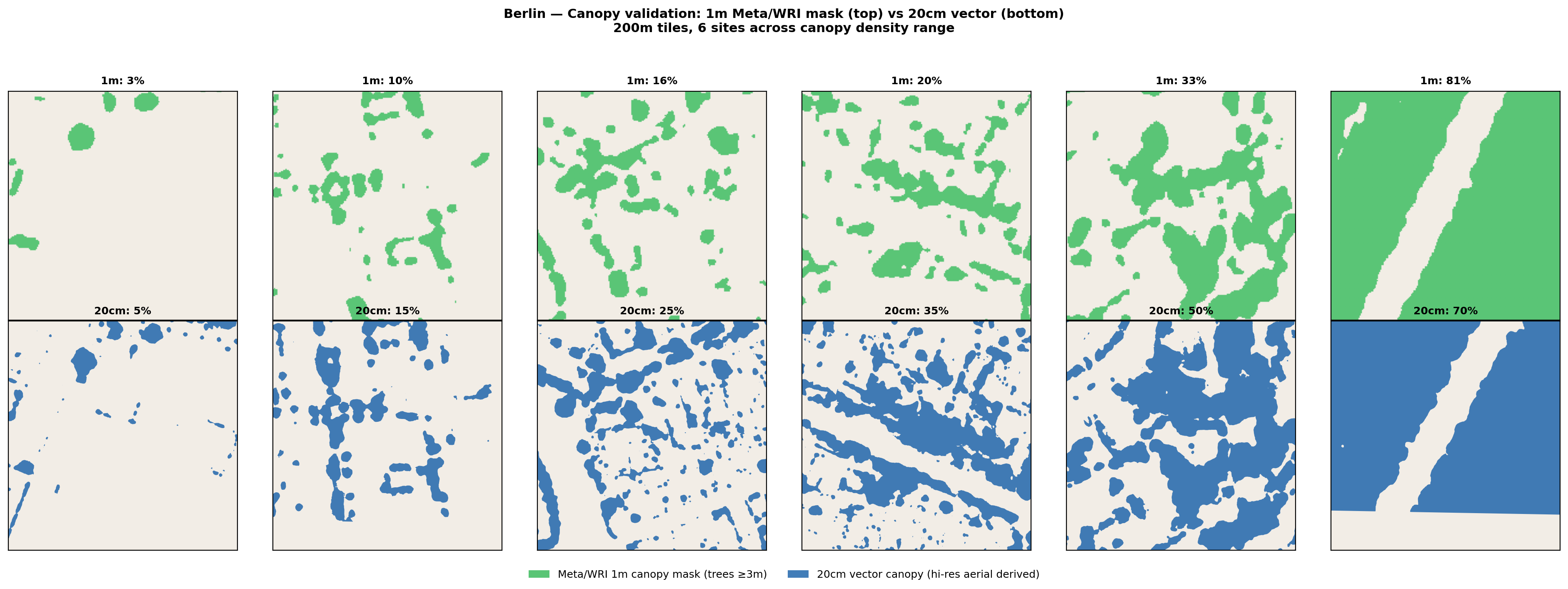
The 1m Meta/WRI canopy product was validated against independently derived 20cm resolution vector canopy data for Berlin and London. The 20cm product was generated from high-resolution aerial imagery using automated tree detection, providing a higher-fidelity reference for canopy area estimation.
Berlin validation
London validation
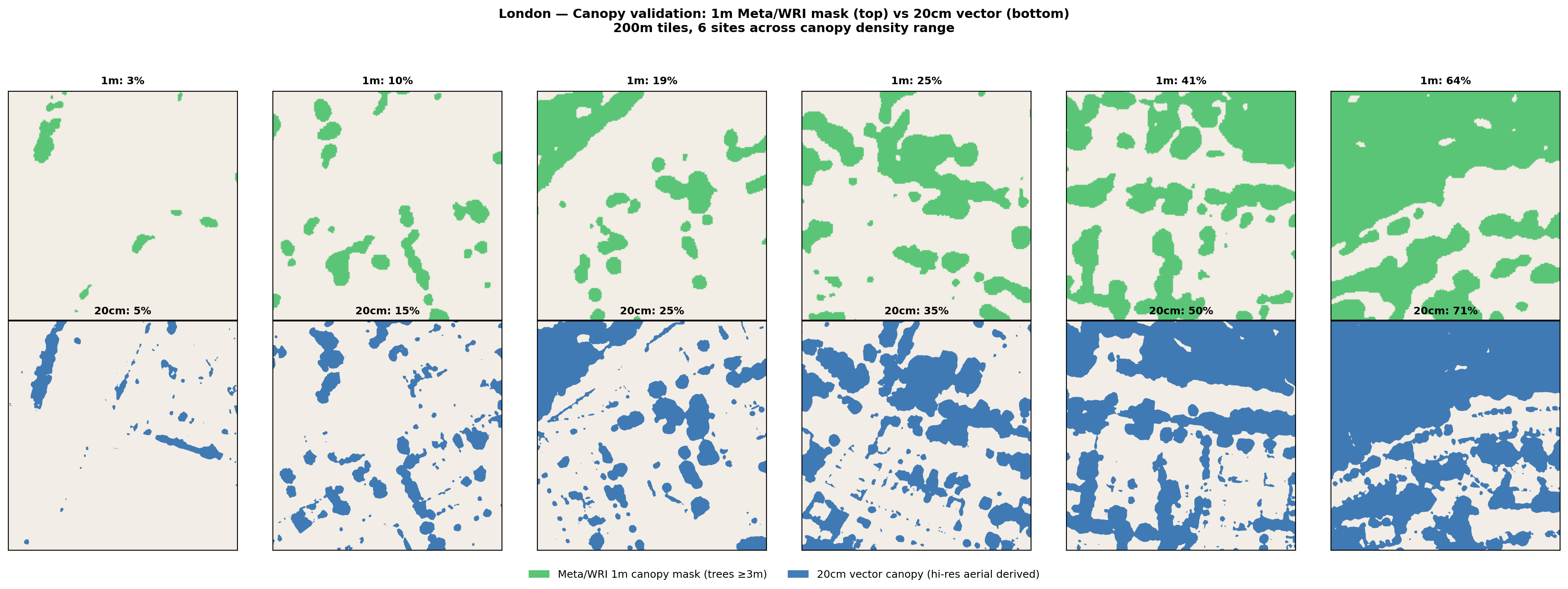
Key finding: The 1m Meta/WRI product underestimates canopy area by approximately 5–15 percentage points compared to the 20cm reference, particularly in the 15–50% canopy range. This is expected: the coarser resolution misses narrow tree crowns, street trees, and small garden trees that are resolved at 20cm. At very high canopy density (>60%), the products converge or the 1m product slightly overestimates due to crown overlap effects.
Implication for this analysis: The canopy deficit figures presented here are likely conservative. If anything, there is slightly more canopy than the 1m product detects, meaning the true cooling gap may be marginally smaller, but the overwhelming finding (>90% of buildings below threshold) holds robustly. The 30% threshold applied in this analysis corresponds to roughly 35–40% in the 20cm product, still well within the range identified in the cooling literature.
Canopy resolution and height filtering
The canopy data used in this analysis comes from two sources at different resolutions. The interaction between resolution, height filtering, and vegetation classification has important implications for interpreting the results, and we want to be fully transparent about the choices made.
Two canopy products. The primary canopy source is the Meta/WRI Global Canopy Height model (1m resolution, 2020 imagery). For eight cities (Berlin, Birmingham, Hamburg, Leeds, Liverpool, London, Munich, Newcastle), we have obtained 0.2m resolution canopy classifications from Google’s Environmental Insights Explorer (EIE) data via Google Earth Engine (imagery mostly 2022–2024, range 2020–2024). We are progressively replacing the 1m product with 0.2m data as it becomes available; additional cities are in processing.
What the 0.2m product measures, and what it doesn’t. The 0.2m EIE product uses a fundamentally different approach from the Meta/WRI height model. According to Google’s published methodology, it is a machine learning classification of high-resolution aerial imagery: an AI model trained to examine pixels and categorise them into terrain types (e.g. “tree,” “road,” “building”). The tree canopy percentage is then the ratio of pixels classified as “tree” to the total number of pixels within a given boundary. This is an image classification task, not a height measurement: the model identifies trees by visual pattern (texture, colour, canopy shape) rather than by measuring their physical height.
This means the 0.2m product resolves individual tree crowns, street trees, and garden features at very high spatial resolution, but it classifies based on what looks like a tree from above. Google notes that results can differ from ground-level surveys or LiDAR-based methods, and recommends visual verification against the interactive map. The model may classify some non-tree vegetation (dense hedgerows, large shrubs) as “tree” if it presents a tree-like canopy pattern from above, and may miss trees that are obscured or recently planted.
This is a meaningful distinction from the Meta/WRI product. The cooling literature (Ziter et al. 2019, the 3-30-300 rule) refers specifically to tree canopy, i.e. shade from overhead foliage. The EIE model is trained to identify trees specifically, but as an image classifier it cannot perfectly distinguish a dense 2m-tall hedge from a low-branching tree. The 30% threshold we apply was calibrated for tree canopy, and applying it to an ML classification that may include some non-tree features lowers the bar slightly.
What the 1m Meta product measures. The Meta/WRI product provides continuous canopy height estimates. Our initial analysis applied a ≥3m height filter, following the product’s intended use case. This filter excludes vegetation that may provide some shade but falls below the canopy height typically associated with sustained cooling. However, the 1m resolution means that small-crowned trees, narrow street trees, and garden trees can be missed entirely, since a single 1m pixel may average a tree crown with adjacent ground and fall below the detection threshold.
A deliberately generous approach. We have adopted the more inclusive method (all detectable vegetation, without height filtering) as the primary measure. This is a conscious choice to err on the side of generosity toward cities. The reasoning:
- Cities that fall short of the 30% threshold even under this generous measure are almost certainly performing worse in reality, since the measure includes low vegetation that provides little shade.
- This approach avoids the opposite risk of the height-filtered method: penalising cities for having young trees, recently planted street trees, or lower-growing species that are still contributing to urban cooling.
- The direction of bias is transparent and consistent: our canopy figures are upper-bound estimates, not lower-bound.
Uncertainties this introduces:
- The EIE product (0.2m) is trained to identify trees, but as an image classifier it may misclassify some dense hedgerows or large shrubs as tree canopy if they present a tree-like pattern from above. Google recommends visual verification and notes that results can differ from ground-level surveys. However, the model is specifically trained on tree identification; it is not a generic “greenness” measure.
- The 1m Meta/WRI product (unfiltered) counts all pixels with any detected vegetation height > 0. This is genuinely a broader measure than tree canopy: it includes hedgerows, shrubs, and ground-level vegetation. The 30% threshold was developed for tree canopy specifically, so some buildings may cross the threshold on the strength of non-tree vegetation.
- Cross-product consistency: the two products use fundamentally different methods (ML image classification vs. height model reclassification). Where both are available, they produce broadly consistent results at the neighbourhood scale, but individual buildings may differ.
- For cities still using the 1m product, the coarser resolution inflates canopy coverage because 1m pixels containing partial tree crowns register as fully vegetated. The 0.2m product avoids this by resolving crowns more precisely.
- Cities with extensive low vegetation (Mediterranean gardens, hedgerow-rich suburbs) may appear greener under the 1m unfiltered product than their shade provision warrants. The EIE product is less susceptible to this because it classifies tree-like features specifically, not all vegetation.
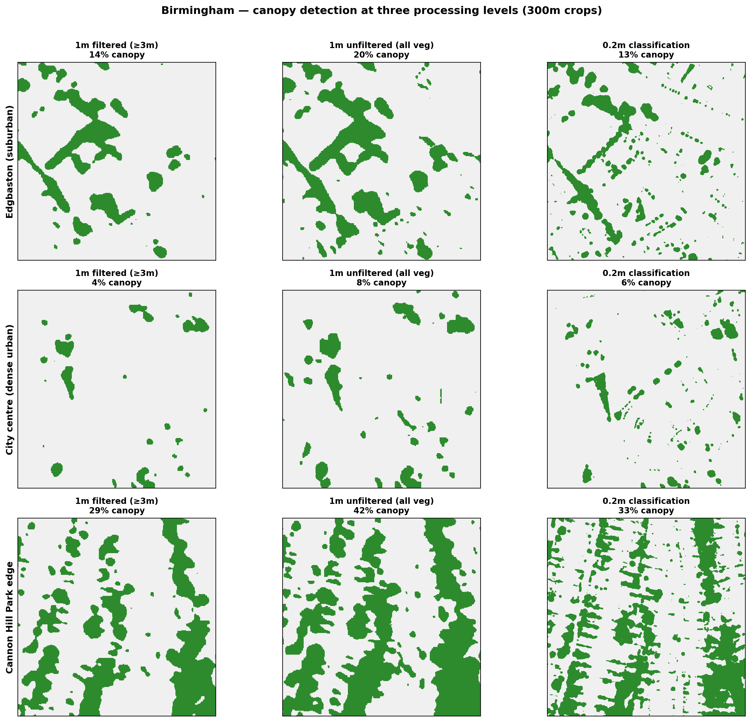
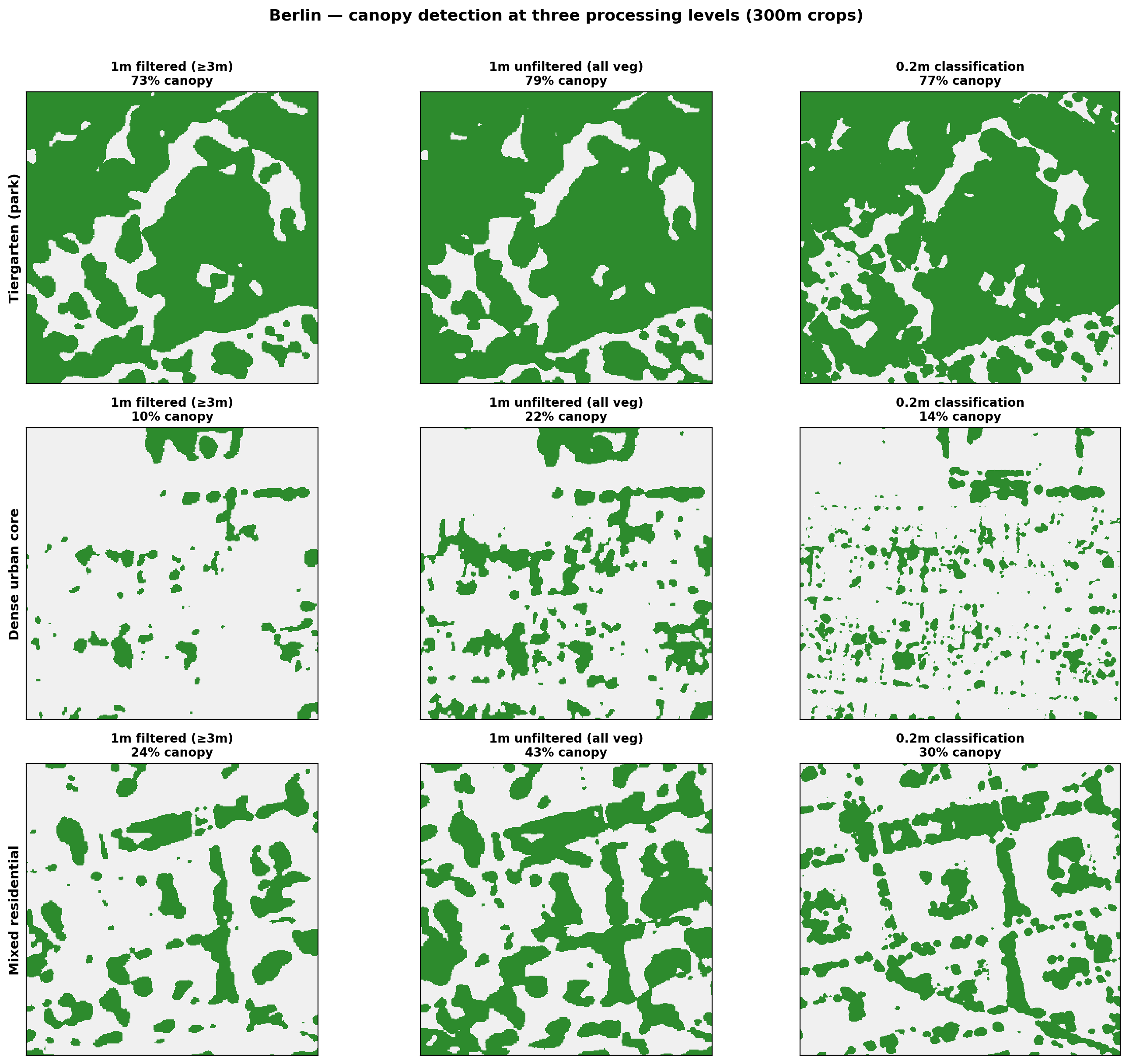
Comparing the three processing levels. To illustrate the differences between products, we compared three versions of the canopy data for the same locations: (1) 1m Meta product with ≥3m height filter, (2) 1m Meta product without height filter (all detected vegetation), and (3) 0.2m EIE ML classification.
Birmingham
| Location | 1m filtered (≥3m) | 1m unfiltered (all veg) | 0.2m classification |
|---|---|---|---|
| Edgbaston (suburban) | 14% | 20% | 13% |
| City centre (dense urban) | 4% | 8% | 6% |
| Cannon Hill Park edge | 29% | 42% | 33% |
Berlin
| Location | 1m filtered (≥3m) | 1m unfiltered (all veg) | 0.2m classification |
|---|---|---|---|
| Tiergarten (park) | 73% | 79% | 78% |
| Dense urban core | 10% | 22% | 14% |
| Mixed residential | 24% | 43% | 30% |
Key observations:
- In park areas (Tiergarten, Cannon Hill), all three products converge: mature canopy is captured regardless of method or resolution.
- In dense urban areas, the 1m unfiltered product roughly doubles the filtered result, because coarse pixels amplify small vegetation features. The 0.2m product sits between the two: it detects more than the filtered 1m but without the pixel-smearing inflation.
- In mixed residential areas, the 0.2m product detects substantially more vegetation than the 1m filtered version (e.g. 30% vs 24% in Berlin, 33% vs 29% in Birmingham), largely resolving garden trees and hedgerows that the coarser product misses.
Impact on headline results. The effect of switching to the 0.2m product varies by city. For Birmingham, changes are modest: the proportion below 30% canopy shifted from 95.1% (1m filtered) to 95.2% (0.2m), and mean canopy moved from 13.6% to 11.7%. For Berlin, the shift was much larger: 80.0% below threshold (1m filtered) dropped to 49.1% (0.2m). This reflects Berlin’s extensive courtyard gardens, allotments, and distributed low vegetation that the 1m product systematically undercounts. Mean canopy remained at 21.0%, indicating that the additional detected vegetation is concentrated among buildings that were near the threshold (pushing many of them above 30%) rather than changing the citywide average.
Implication for readers. The canopy percentages reported here should be understood as an upper-bound estimate that includes all detectable vegetation, not just shade-providing trees. Where cities fall below the 30% threshold under this generous measure, the deficit relative to the cooling literature’s recommendations is likely larger than the numbers suggest. We are progressively replacing 1m data with 0.2m data to improve spatial precision; this may shift headline numbers for individual cities but does not change the overall finding across the dataset.
Spatial coverage and hybrid analysis
The 0.2m canopy rasters are exported from Google Earth Engine as square tiles. The data footprint within each tile does not always cover the full city boundary used to extract building footprints. Where the 0.2m raster has no data, buildings would either receive artificially inflated canopy percentages (if nodata pixels are excluded from the calculation) or be assigned zero canopy (if treated as missing). Neither is acceptable.
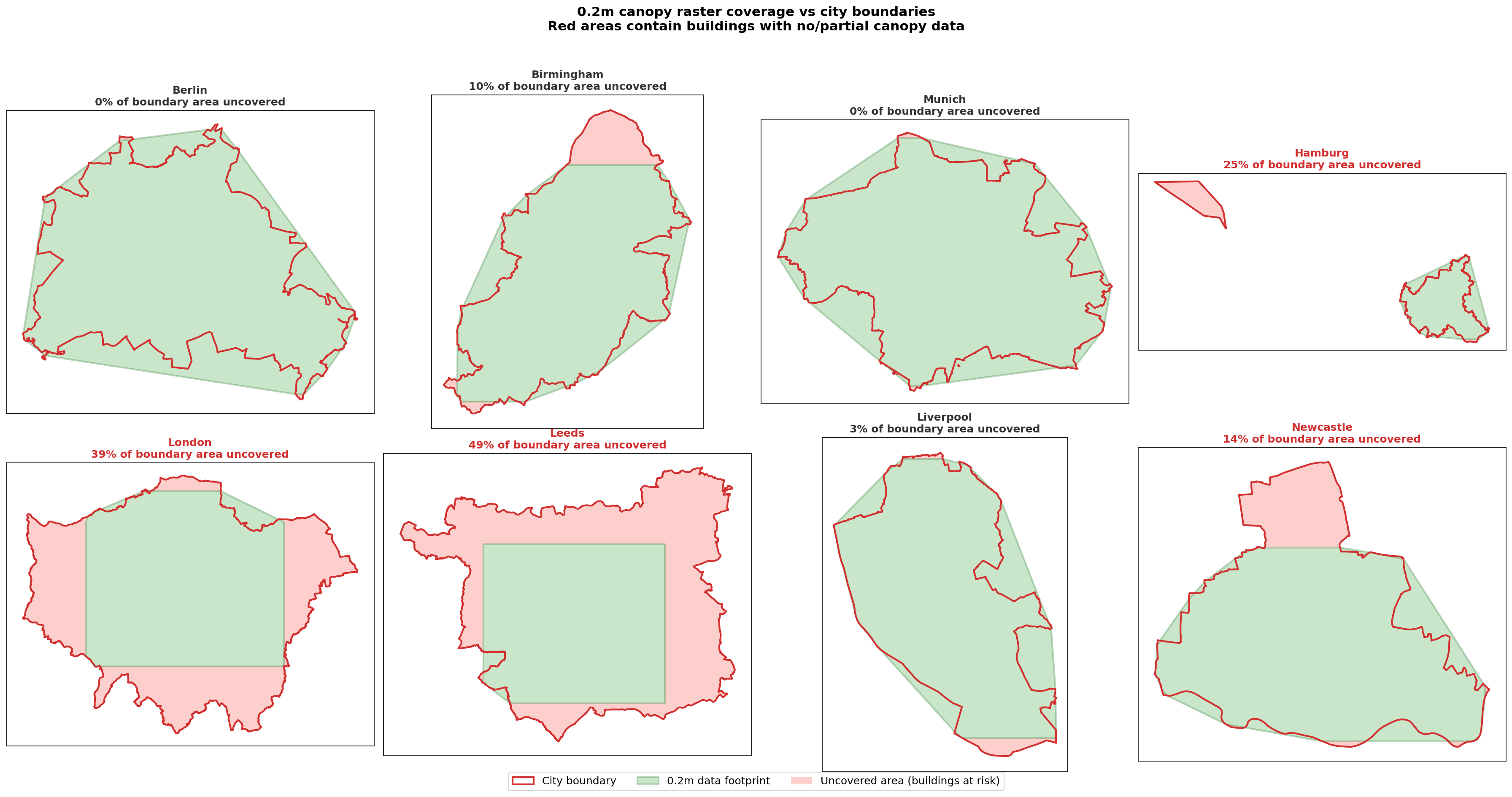
We addressed this by adopting a hybrid approach for cities where the 0.2m product does not fully cover the city boundary:
- Buildings within the 0.2m data footprint use the 0.2m canopy classification.
- Buildings outside the 0.2m footprint fall back to the 1m Meta/WRI product (without height filtering), which has verified full coverage across all city boundaries.
This affects Birmingham (5.5% of buildings outside footprint), London (27.8%), Leeds (25.5%), and Newcastle (2.3%). For Munich, Berlin, Hamburg, and Liverpool, the 0.2m product covers the boundary adequately and no hybrid fill is needed.
Each building is tagged with its canopy data source (canopy_source = “0.2m” or “1m_unfiltered”), enabling transparent reporting. The map below shows the spatial distribution of data sources for the four hybrid cities:
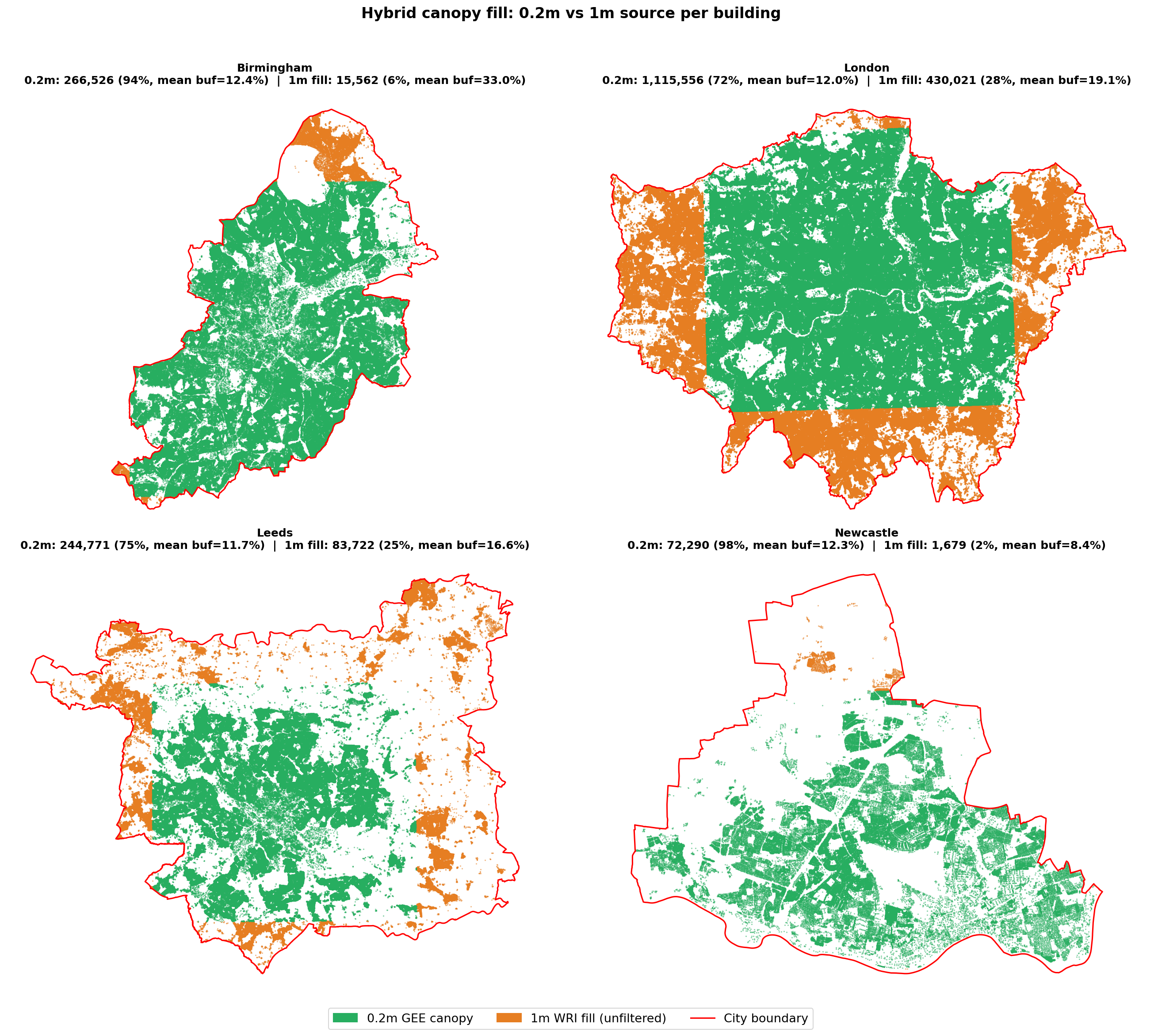
The 1m fallback uses the same all-vegetation measure as the 0.2m product: any detected vegetation height > 0 counts as canopy, with no height filter. In the overlap zone where both products have data, they produce consistent results (see three-layer comparison above), so the transition does not introduce a visible discontinuity.
Threshold justification
The 30% canopy threshold is based on peer-reviewed evidence:
- Ziter et al. (2019) found that cooling effects of urban tree canopy become significant above approximately 30–40% coverage within the local vicinity. The 30% threshold is also proposed as a general bare minimum for urban forest in cities as part of the 3-30-300 rule.
- The 60m buffer distance from each building outline corresponds to the neighbourhood-scale at which canopy-mediated cooling is detectable in surface and air temperature measurements.
Landsat scene table
| City | Scene date | Notes |
|---|---|---|
| Marseille | 2024-08-05 | Summer heatwave |
| Rome | 2024-07-17 | Summer heatwave |
| Naples | 2024-08-11 | Summer heatwave |
| Madrid | 2024-07-23 | Summer heatwave |
| Milan | 2024-07-15 | Summer heatwave |
| Toulouse | 2024-08-10 | Summer heatwave |
| Nice | 2024-07-29 | Summer heatwave |
| Barcelona | 2024-07-27 | Summer heatwave |
| Munich | 2024-07-31 | Summer heatwave |
| Berlin | 2025-07-01/02 | Max composite, 3 scenes across paths 193+194 (99.96% coverage) |
| Cologne | 2024-08-28 | Summer heatwave |
| Lyon | 2022-08-07 | 2022 scene (cloud cover in 2024) |
| Paris | 2024-08-26 | Summer heatwave |
| Lisbon | 2024-09-14 | Late summer |
| Athens | 2024-08-03 | Summer heatwave |
| London | 2026-05-26 | May 2026 (most recent clear pass) |
| Porto | 2024-09-14 | Late summer |
| Thessaloniki | 2024-07-16 | Summer heatwave |
| Bristol | 2026-05-24 | May 2026 |
| Birmingham | 2026-05-24 | May 2026 |
| Leeds | 2024-07-30 | Partial cloud cover (14.4%) |
| Liverpool | — | No suitable scene selected |
| Newcastle | 2023-09-05 | Late summer |
| Sevilla | 2023-07/08 | Max composite, 10 scenes across paths 201+202 during Iberian heatwave (100% coverage) |
| Hamburg | 2023–2024 | Median composite, 38 summer scenes across multiple paths (98% coverage) |
Data sources
| Input | Source | Resolution | Vintage | Access |
|---|---|---|---|---|
| Tree canopy height | Meta/WRI Global Canopy Height | 1m | 2020 | Google Earth Engine |
| Tree mask (all vegetation) | Derived from canopy height (no height filter) | 1m | 2020 | — |
| Hi-res tree canopy | Google EIE (ML classification of aerial imagery) | 0.2m | 2020–2024 | Google Earth Engine |
| Hi-res validation canopy | Aerial-derived vector canopy | 20cm | 2024 | Berlin Senate / Ordnance Survey |
| Building footprints (FR) | IGN BD TOPO v3 | Vector | 2024 | data.gouv.fr WFS |
| Building footprints (other) | Overture Maps Foundation | Vector | 2024 | overturemaps.org |
| Land surface temperature | Landsat 8/9 C2L2 ST_B10 | 30m | 2022–2026 | Google Earth Engine |
| Income (FR) | INSEE Filosofi | 200m grid | 2019 | insee.fr |
| Deprivation (UK) | IMD 2025 | LSOA | 2025 | gov.uk |
| Deprivation (DE) | GISD | Municipality | 2020 | rki.de |
Software
Python 3.12, GeoPandas, Rasterio, exactextract, GDAL, NumPy, Matplotlib, contextily, Leaflet.js. Site built with Quarto. Maps rendered using CartoDB Positron basemap tiles.
Code availability
Analysis code is available at github.com/tcroeser/EU_Heatwave_Explorers.
Unpublished spatial analysis by Dr Thami Croeser, June 2026. This analysis was conducted independently to support the above comment article. The data, methods, and findings are the sole responsibility of the analyst.